
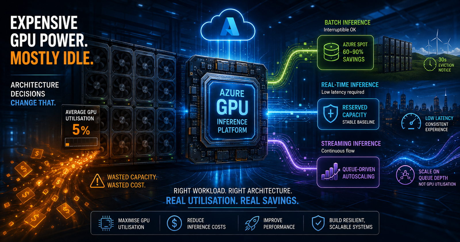
Across more than 23,000 production Kubernetes clusters running AI workloads on AWS, Azure and GCP, average measured GPU utilisation was just 5 percent. On AKS specifically, it averaged just 2 percent. That figure comes from Cast AI’s 2026 State of Kubernetes Optimization Report, and it should reframe how most platform teams think about Azure GPU inference costs: the discount model you choose for a GPU VM matters far less than whether that GPU is doing any work at all.
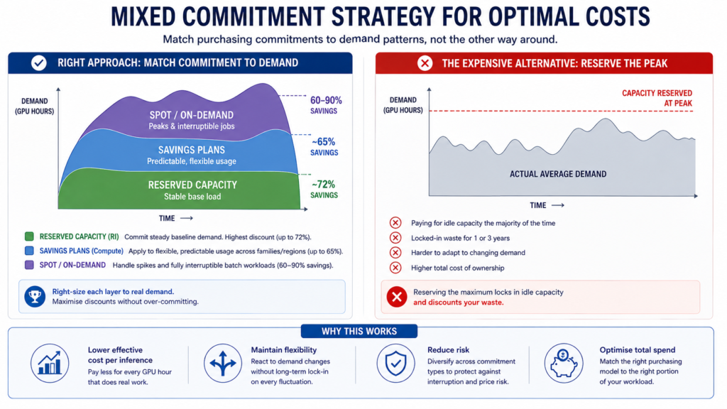
Most organisations respond to rising inference bills by shopping for a cheaper SKU or negotiating a bigger reservation. That instinct is understandable and largely wrong. A team that reserves an ND H200 v5 node for three years and then runs it at 5 percent utilisation has locked in a 65 percent discount on the existing utilisation pattern, not a fix for it: the reservation discounts the waste rather than removing it. The traditional approach, buy the discount first and architect later, treats GPU inference like a fixed-capacity problem when it is actually a scheduling and batching problem wearing a hardware costume. Reserved Instances and Savings Plans are real levers, worth up to 72 percent and 65 percent respectively against pay-as-you-go, but they compound whatever utilisation pattern already exists rather than fixing it.
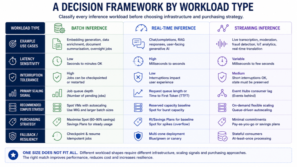
The alternative is to stop treating “GPU inference” as one workload and start treating it as three: batch, real-time and streaming, each with a different tolerance for interruption and a different cost lever as a result. Batch inference can absorb Azure Spot’s 30-second eviction notice and save 60 to 90 percent. Real-time serving cannot, and needs a reserved floor with Spot only for burst capacity. Streaming inference needs neither discount model as its primary lever; it needs autoscaling on queue depth rather than GPU utilisation, because utilisation alone hides how loaded an LLM serving layer actually is. One verified GPU deployment and one managed-endpoint validation example below, one in energy, one in UK insurance, show what parts of this look like in practice. This piece sets out the architecture, the numbers and a decision framework for getting there.
Why Azure’s GPU Fleet Looks Different in 2026
Azure’s GPU line-up for inference has matured considerably since the A100 generation. The NCads H100 v5 series, generally available since March 2024, offers one- or two-GPU configurations of the H100 NVL card with 94 GB of HBM3 each, paired with fourth-generation AMD EPYC Genoa, and is Azure’s mainstream option for this class of hardware. It is not the only single-GPU H100 series: the confidential-computing NCCads H100 v5 series also ships a single H100 NVL GPU inside a Trusted Execution Environment, for workloads that need hardware-isolated inference rather than raw throughput. Microsoft’s own general availability announcement states that customers will experience between 1.6 and 1.9 times the inference performance of the previous NC A100 v4 generation depending on workload type, and positions the mainstream series for batch inferencing with heavy pre- and post-processing and applied AI development. For teams whose models fit comfortably on a single GPU, NCads H100 v5 is now the default inference SKU rather than the older NC A100 v4.
Above it sits the ND H200 v5 series, generally available in late 2024: eight H200 GPUs per VM, 141 GB of HBM3e each, 4.8 TB/s of memory bandwidth per GPU and Quantum-2 InfiniBand tying the nodes together. Microsoft measured up to 35 percent higher inference throughput than ND H100 v5 on Llama 3.1 405B in its own tested configuration, which used a larger batch size on H200, suggesting the additional HBM capacity contributed materially to the result rather than raw compute alone. That distinction matters for architecture decisions: when HBM capacity, not FLOPS, is the bottleneck, moving to H200 is a batching upgrade as much as a hardware upgrade. The ND MI300X v5 series, AMD’s answer, offers 192 GB of HBM3 per GPU, more than Azure’s H100 or H200 options, and is the SKU of choice when fitting a 70-billion-parameter-plus model on fewer GPUs matters more than NVIDIA’s software ecosystem. It is no longer Azure’s largest per-GPU memory footprint, though: the newer ND GB300 v6 series (Blackwell Ultra) reaches 288 GB of HBM3e per GPU. At the top of the mainstream range, ND GB200 v6 brought Blackwell into general availability for frontier-scale generative inference. Microsoft’s own benchmark reports a 2.45 times increase in theoretical peak FP8 throughput over H100 per GPU (4,856 versus 1,979 TFLOPS), with a measured, sustained FP8 result of roughly double the H100 once real-world conditions such as warm-up and memory access patterns are accounted for, still a substantial gain, just a smaller one than the peak figure alone suggests.
The common thread across this generation is that Azure has quietly built the complete guide to choosing the right Azure VM series worth revisiting for GPU workloads specifically, because the old heuristic of “biggest GPU you can afford” no longer holds. Microsoft’s own benchmarks show substantial, workload-dependent gains for NC H100 v5 over the previous NC A100 v4 generation rather than a universal claim against any specific prior configuration, and choosing the eight-GPU ND-series when a workload does not need multi-node InfiniBand is a common and expensive over-provisioning mistake regardless of which generation is involved.
The underlying NVIDIA generation timeline is worth holding in mind when planning a multi-year architecture: H100 reached Azure general availability in 2024, H200 followed within the same year, and Blackwell-based GB200 and GB300 hardware arrived through 2025 and into 2026. Azure’s accelerator portfolio is turning over quickly enough that a three-year Reserved Instance commitment can comfortably span at least one major hardware refresh, which argues for shorter commitment terms on the newest SKUs and longer terms only where a workload is confident it will still be running on that specific hardware generation in three years. Regional pricing also varies more than many teams expect, though the exact gap moves with demand and should always be checked in the Azure Pricing Calculator rather than assumed. Third-party pricing trackers have observed East US as consistently among the cheapest regions for GPU SKUs, with West US 2, Europe West, and especially Southeast Asia and Australia East running meaningfully higher for equivalent H100 capacity at various points through 2026. A workload with data residency flexibility can save meaningfully just by checking region before choosing discount model.
The other structural shift is on the discount side. Both Azure and AWS can interrupt Spot capacity for capacity reclamation and, in each case, when the Spot price exceeds a configured maximum, so eviction triggers are broadly similar across the two platforms. The genuine operational difference is the notice period: Azure Spot Virtual Machines give as little as 30 seconds, materially shorter than the two-minute warning AWS normally gives EC2 Spot customers before a stop or termination. This is not a minor implementation detail. It is the single constraint that should determine whether a workload is Spot-eligible at all, and it is precisely the class of comparative claim that gets glossed over in vendor pricing pages. Teams migrating fault-tolerant patterns from AWS to Azure, including the ones described in our Spot Instance Architecture piece, need to rebuild checkpoint intervals around a much tighter eviction window, not simply port over an AWS-tuned design.
Technical Architecture for GPU Inference on Azure
Managed endpoints versus self-managed AKS
Azure Machine Learning gives two serving primitives that sit at opposite ends of the control spectrum. Managed online endpoints run behind Azure Monitor-based autoscaling, support GPU compute, and provide managed deployment infrastructure with configurable blue-green, mirrored-traffic and gradual rollout patterns, but they do not scale to zero, so a minimum replica count sits on the bill continuously. Managed batch endpoints are the mirror image: they scale to zero between jobs and divide work into batches that can be retried on interruption, and cost nothing beyond the underlying compute, since Azure Machine Learning adds no service charge on top of the VM price. Retry is not the same as application-level checkpointing, though, so anything that cannot safely be recomputed after an interruption should still be persisted by the application itself.
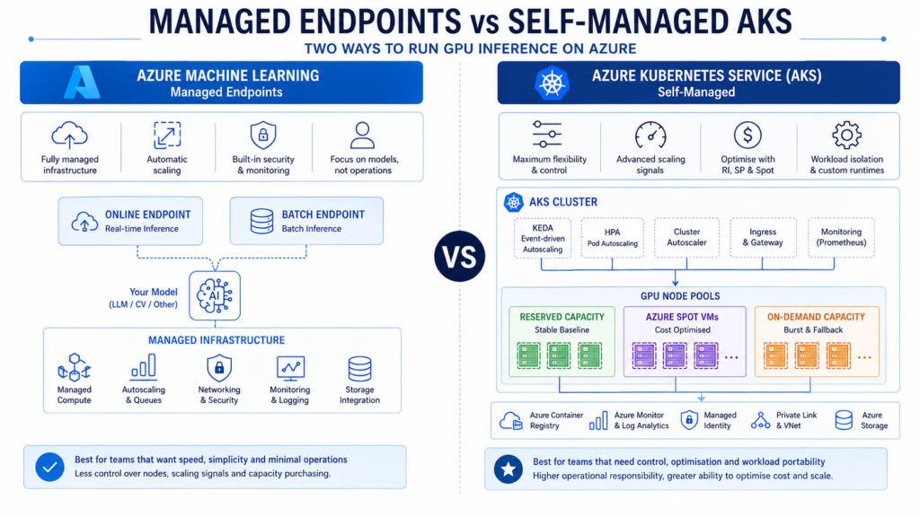
AKS trades that operational simplicity for control. The production-grade AKS patterns we covered previously apply directly here: GPU node pools with the NVIDIA device plugin, Multi-Instance GPU partitioning on A100, H100 and now H200 series hardware, and KEDA scaling GPU-consuming workloads down to zero replicas, with the cluster autoscaler or AKS Node Auto Provisioning then removing the resulting idle nodes where the node-pool configuration supports it. These are two separate control loops working together, not one, and the distinction matters because it does not hold uniformly across every AKS GPU configuration. The trade-off is real in three specific ways. Fully managed AKS GPU node pools remain in preview and do not support the cluster autoscaler during that preview, so they must be scaled manually, with AKS Node Auto Provisioning as a separate provisioning path for teams that need it. MIG profiles are fixed at node-pool creation and require a drain-and-recreate cycle to change. And, as of this writing, the cluster autoscaler does not natively scale mixed MIG-profile node pools because the underlying nvidia.com/gpu resource naming does not distinguish between MIG partition sizes. Teams that need both memory partitioning and elastic scaling should plan MIG pools as fixed-size for now and layer KEDA-driven, non-MIG pools around them for the elastic portion of demand.
Multi-Instance GPU and dynamic batching
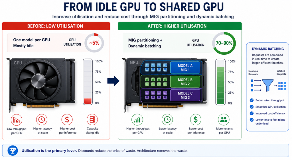
MIG matters because it addresses the utilisation problem directly rather than through pricing. A single H100 or H200 partitioned into MIG slices lets several inference workloads share one physical GPU with hardware-level memory and fault isolation, which is exactly the fix for a workload that needs a fraction of a GPU’s compute but historically had to reserve the whole card. Combined with dynamic or continuous batching in the serving engine itself, tools such as vLLM or NVIDIA Triton, and FP8 quantisation where model accuracy permits, these are first-order levers on the utilisation side of the equation. Cast AI has published a single observed case of a 136-node H200 inference fleet reaching 49 percent average utilisation, roughly ten times the fleet-wide average in the same report, which the vendor attributes largely to serving technique rather than to different hardware. It is one vendor-reported example rather than a controlled comparison, but directionally it supports the same point this section makes on other grounds: batching and partitioning are worth investigating before assuming a different SKU is the answer.
Autoscaling signals by workload shape
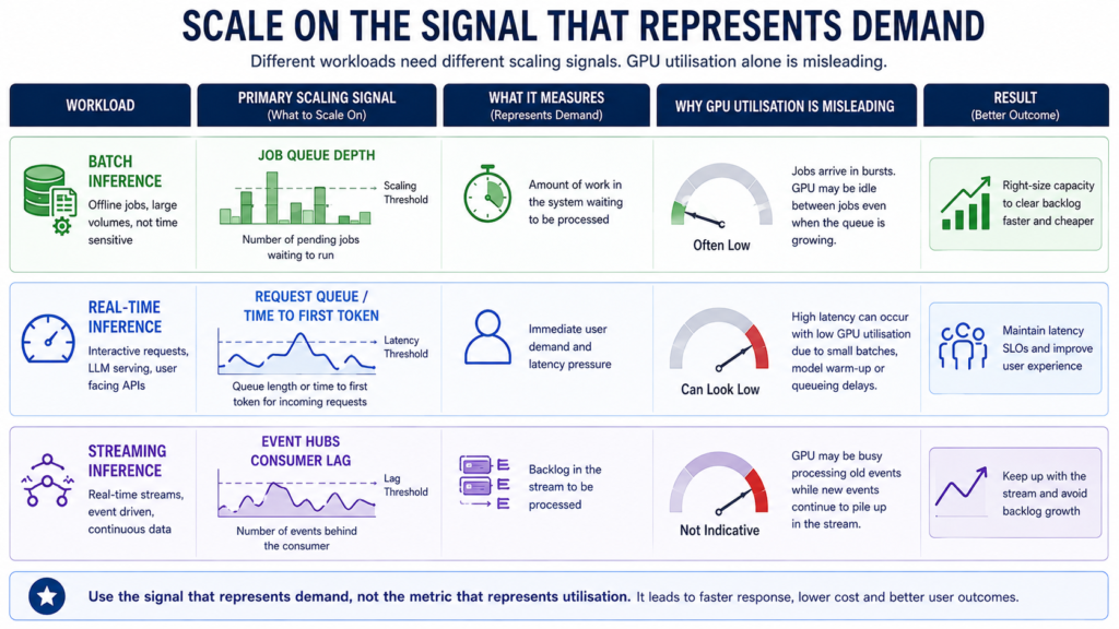
The single biggest architectural mistake in GPU inference deployments is scaling on the wrong signal. GPU or CPU utilisation under-represents LLM load because inference has distinct prefill and decode phases with very different resource profiles, so a workload can be saturated on latency while utilisation graphs look calm. Microsoft’s own guidance for NVIDIA Dynamo on AKS recommends scaling on time-to-first-token latency at the 95th percentile, or on queue depth, rather than on raw GPU utilisation. For streaming workloads fed by Azure Event Hubs, the equivalent signal is consumer group lag: KEDA’s Event Hub scaler reacting to backlog depth is the correct trigger, not CPU or GPU load on the consuming pods. Getting this signal wrong produces two failure modes in roughly equal measure: over-provisioned pools that sit idle waiting for a spike, and under-provisioned pools that look healthy on a dashboard while user-facing latency quietly breaches its service level.
Comparing the Serving Approaches
No single serving pattern is correct across all three workload types, which is why the comparison below is organised by what each approach optimises for rather than by which vendor built it.
| Approach | Scale-to-zero | Typical latency profile | Operational effort | Best fit |
|---|---|---|---|---|
| AML managed online endpoint | No (minimum replicas required) | Low, consistent | Low | Real-time serving where ops capacity is limited |
| AML batch endpoint | Yes, between jobs | Not latency-sensitive | Low | Batch inference, especially with unpredictable job cadence |
| AKS with KEDA and cluster autoscaler | Yes at the pod level via KEDA, and at the node level via cluster autoscaler or Node Auto Provisioning where supported | Depends on warm floor configured | High | Any workload type, when fine-grained control justifies the overhead |
| AKS with MIG | No (fixed partition size; cluster autoscaler does not scale mixed MIG profiles) | Low, isolated per partition | High | Sub-GPU real-time workloads with stable demand |
| Azure Container Apps serverless GPU | Yes | Cold start typically tens of seconds on supported T4 and A100 hardware | Low | Lightweight models, roughly under 13 billion parameters as a rough guide that varies with quantisation and context length |
Managed AML endpoints win on operational simplicity and are the right default for teams without a platform engineering function dedicated to Kubernetes. AKS wins on cost efficiency at scale precisely because KEDA and cluster autoscaler expose every lever, queue depth, custom Prometheus metrics, scheduled scaling, that managed endpoints abstract away. Azure Container Apps’ serverless GPU tier fills a real gap for models small enough to tolerate a short cold start, avoiding both the AML minimum-replica cost and the AKS operational overhead entirely.
The comparison our Cloud AI Platform Showdown piece ran across GCP, AWS and Azure ML still holds at the platform level: Azure’s differentiator for GPU inference specifically is not any single managed service but the breadth of the AKS ecosystem around it, MIG, KEDA, KAITO, NVIDIA Dynamo integration, which in our view gives Azure customers a wider set of architectural options to choose from than the managed-endpoint layer alone would suggest, even if a like-for-like comparison against every equivalent AWS and GCP tool is beyond the scope of this piece.
Azure Examples: OriGen’s GPU Deployment and AXA UK’s Managed-Endpoint Validation
Company Name and Industry: OriGen, Energy software (oil and gas reservoir simulation)
Scale Context: Historical production matching across a Colombian oilfield spanning thousands of wells and 40 years of data, for customer Ecopetrol
Challenge: Traditional CPU-based reservoir simulation required thousands of individual runs, each taking hours to days, to reach an accurate prediction
Solution Implemented: Physics-informed neural networks served on NVIDIA GPU-accelerated Azure VMs (NCas T4 v3, NCv3 and NC A100 v4 series), orchestrated through Azure Kubernetes Service with Azure Blob Storage for data loading, deployed as a multi-tenant SaaS platform
Measurable Outcomes:
- Single simulation time reduced from hours or days to milliseconds, a reported 1,000-fold speed increase
- 85 percent match rate achieved across more than 1,000 wells in the history-matching exercise
- Customers report materially faster time to production decisions on well yield and injection planning
Company Name and Industry: AXA UK, Insurance (validation example, not a confirmed production GPU deployment)
Scale Context: 30 million car insurance quotes served daily via aggregator and broker sites, at a required throughput of 400 quotes per second
Challenge: The pricing team needed to validate faster deployment of new pricing models without sacrificing the sub-second response time the aggregator business model depends on
Solution Implemented: Testing and validation of a PaaS environment on Azure Machine Learning using managed online endpoints, with both natively-built and ONNX open-source models evaluated ahead of a planned early-2022 production go-live
Measurable Outcomes (from testing, not confirmed production operation):
- Response time requirement of 200 milliseconds met in testing under managed endpoints
- Optimised response time reduced to as low as 130 milliseconds in testing, a reduction of roughly 60 percent against the prior benchmark
- Microsoft’s published story states the company was not yet running the new models in production at time of writing, with go-live planned for early 2022, so these are validation results rather than a measured post-deployment outcome
The AXA UK story does not specify whether its pricing models were tested on GPU or CPU compute, and, as Microsoft’s own published version of the story makes clear, testing had been completed but production go-live had not, at time of publication. It is included here as evidence for the managed-endpoint architecture pattern under real throughput and latency constraints, not as a verified GPU deployment. OriGen’s story is the only one of the two that confirms customer-operated GPU hardware, AKS orchestration and a measured, in-production outcome.
Cost Analysis and Return on Investment
List prices for Azure’s current GPU generation vary meaningfully by SKU and region, and change often enough that any figure printed here should be treated as illustrative rather than a number to budget against. Third-party pricing trackers, not Azure’s own published rate card, put a single-GPU NC40ads H100 v5 on-demand at somewhere in the region of $7 to $8.30 an hour in East US, with the spread reflecting different capture dates rather than a single settled price. A multi-GPU ND96isr H100 v5 configuration has been tracked in the region of $90 to $100 an hour on-demand. Capture a dated export from the Azure Pricing Calculator or the Azure Retail Prices API for the specific SKU, region and date relevant to a real business case rather than relying on any single published figure, including these.
Three discount mechanisms layer on top of list price, and each earns its keep on a different slice of demand, though the headline percentages below are Microsoft’s own generic worked examples on non-GPU VM sizes and should be confirmed against the specific GPU meter and region before being used in a business case. Reserved Instances save up to 72 percent against pay-as-you-go on a one or three-year term, based on Microsoft’s published example using a 36-month commitment. Azure Savings Plans save up to 65 percent, are OS and region-flexible, and cover AKS, App Service and Functions consumption alongside raw VM spend, and are generally treated as a fixed commitment for the term once purchased. Spot Virtual Machines save 60 to 90 percent depending on SKU, region and how tightly the workload can tolerate the 30-second eviction window. Reserved Instance eligibility is also worth checking per SKU rather than assumed: Microsoft has already withdrawn new Reserved Instance purchases and renewals for a number of older, non-GPU VM families from July 2026, which is a useful reminder that commitment eligibility can change and should be verified for the exact GPU meter in question before purchase. The standard FinOps layering pattern, familiar from our FinOps Evolution piece, applies directly to GPU fleets: Reserved Instances for the always-on floor, Savings Plans sized against the flexible remainder, Spot for everything interruptible.
Hidden costs deserve more attention than they typically get in inference cost models. Microsoft’s own startup guidance names GPU idle time as the largest hidden cost in self-hosted inference, an unattended A100 running overnight costs more than a month of a small managed database, alongside data egress running 2 to 15 percent of total spend and model artifact storage adding a further 3 to 10 percent. None of these show up on a per-hour SKU comparison, and all of them are why the Cast AI utilisation figures matter more to the total bill than any single discount percentage.
Over a three to five year horizon, the arithmetic favours a mixed commitment strategy over either extreme. A workload committed entirely to on-demand pricing pays the full list price indefinitely and gains only flexibility it may never use. A workload committed entirely to three-year Reserved Instances locks in today’s hardware generation at a fixed rate through at least one and often two NVIDIA generational refreshes, during which newer SKUs may deliver better price-performance than the reserved capacity itself. As a working heuristic rather than a measured finding, the middle path, reserving only the floor that utilisation data confirms is consistently always-on, layering Savings Plans against the next tranche of predictable demand, and leaving burst and batch capacity on Spot or on-demand, is likely to outperform both extremes over a three-year TCO calculation for most fleets. The exact payback period depends heavily on how quickly a given team can raise utilisation from the 5 percent baseline Cast AI observed toward something closer to the 49 percent one of Cast AI’s customer fleets achieved, and should be modelled against real workload data rather than assumed.
A Decision Framework by Workload Type
Classify every inference workload before choosing infrastructure, because the classification determines the architecture far more than the model size does.
Batch inference tolerates the 30-second Spot eviction window because there is no user waiting on the other end of the request. Route it through Azure Batch or AML batch endpoints on Spot-priced GPU capacity, with work broken into short, retryable tasks and application state persisted to Blob Storage between them, since neither service checkpoints application state automatically within a running task. Azure Batch’s low-priority VM tier retired on 30 September 2025, and Microsoft began a system-initiated migration of remaining eligible low-priority pools to Spot in early March 2026, with completion expected within days rather than confirmed as finished at the time of writing, so new batch designs should target Spot directly rather than the retiring tier.
Real-time inference cannot absorb an eviction mid-request without breaching its latency service level, so it needs a warm floor of reserved or on-demand replicas covering baseline traffic, with Spot-backed replicas added only for burst above that floor via KEDA. For LLM serving specifically, prefer time-to-first-token latency or request queue depth as the primary scaling signal, since GPU utilisation under-represents load during the sequential decode phase; for compute-bound, non-LLM inference, DCGM-based GPU utilisation metrics can themselves be an appropriate signal, and Azure’s own KEDA guidance supports scaling directly on GPU utilisation for that case. A full AKS scale-from-zero can take several minutes once node provisioning, container image retrieval and model loading are all counted, though the exact figure depends heavily on SKU, region, image size and model, and should be benchmarked directly rather than assumed. This is why real-time, user-facing workloads should generally avoid true scale-to-zero altogether and retain a warm baseline.
Streaming inference sits between the two: always-on like real-time serving, but elastic in a way batch is not. Ingest through Azure Event Hubs, pre-filter or window with Stream Analytics or Spark Structured Streaming where useful, and feed an AKS GPU deployment scaled by KEDA against consumer group lag rather than against CPU or GPU metrics. The autoscaling signal is the defining architectural choice here, since backlog depth reveals demand that per-pod utilisation figures do not.
As a working heuristic rather than a fixed rule, a workload that tolerates more than roughly ten minutes of end-to-end delay on its worst-case request is a reasonable batch or streaming candidate for Spot capacity. Below that threshold, plan for a reserved floor first and treat Spot as a bonus rather than a foundation.
Risk tolerance should be assessed separately from latency tolerance, because the two do not always move together. A batch workload with a hard regulatory deadline, month-end reconciliation reporting is a common example, has low risk tolerance despite having high latency tolerance, and needs a fallback on-demand pool that activates automatically if Spot capacity is unavailable near the deadline. Conversely, a real-time workload serving an internal tool with generous informal expectations may tolerate more risk than its latency profile suggests, and can run a thinner reserved floor than a customer-facing equivalent. Matching infrastructure to workload type is the starting point; matching the fallback strategy to actual business risk, rather than to the workload’s technical category alone, is what prevents the framework from becoming a rigid checklist.
Implementation Roadmap and What Comes Next
Phase 1, Foundation (Months 1 to 3): Classify existing and planned inference workloads by type, instrument GPU utilisation per workload before any procurement decision, and stand up a single AKS cluster with both a Spot-priced batch node pool and a reserved real-time node pool to validate the pattern against one representative workload of each type. Expect this phase to involve a platform engineer and an ML engineer working jointly, since the classification exercise depends on both infrastructure and model knowledge.
Phase 2, Expansion (Months 4 to 9): Migrate additional workloads into the classified pattern, introduce MIG partitioning for sub-GPU real-time workloads once utilisation data justifies it, and layer Reserved Instances or Savings Plans against the now-stable baseline demand revealed by Phase 1’s instrumentation. This is also the point to move any Event Hub-backed streaming pipelines onto KEDA lag-based autoscaling rather than the CPU-based scaling many teams start with by default.
Phase 3, Maturity (Months 10 to 18): Introduce dynamic batching and quantisation in the serving layer itself for workloads where model accuracy tolerates it, formalise FinOps tagging and idle-GPU alerting across the estate, and revisit commitment levels annually against actual utilisation rather than against the original procurement assumptions.
Looking further out, the direction of travel on Azure is toward tighter coupling between scheduling and inference orchestration rather than toward cheaper raw compute. NVIDIA Dynamo’s integration with AKS, treating the prefill and decode phases as distinct scheduling problems with smart routing and KV cache reuse across nodes, points at where the real efficiency gains are likely to come from over the next eighteen months, alongside broader availability of Blackwell-generation hardware and continued growth in Dynamic Resource Allocation support for finer-grained GPU sharing than MIG’s fixed profiles currently allow.
Strategic Recommendations
Buy less discount and build more classification. The organisations getting genuine value from Azure GPU inference are not the ones with the largest Reserved Instance commitments, they are the ones who can say with confidence which of their workloads is batch, real-time or streaming, and who have autoscaling wired to the metric that actually reflects load for each. A Reserved Instance purchased against an unclassified, poorly-batched workload locks in waste at a discount rather than removing it.
The most common pitfall is treating MIG, KEDA and Spot as interchangeable cost levers rather than as tools for different problems: MIG fixes under-utilised GPUs, Spot fixes overpriced interruptible compute, and KEDA fixes the mismatch between provisioned and actual capacity. Applying only one of the three, most commonly Spot alone, and expecting it to solve all of it, is why so many GPU cost optimisation efforts stall after an initial win. Teams that succeed treat the workload classification as the foundation and layer the pricing mechanics on top of it, not the other way round.
Useful Links
- OriGen: Accelerating Reservoir Simulations with Azure AI Infrastructure
- AXA UK: Insurance Quotes with Azure Machine Learning Managed Endpoints
- Build Workloads with Azure Spot Virtual Machines, Azure Architecture Center
- NCads H100 v5 Series Specification
- NCCads H100 v5 Series Specification (Confidential Computing)
- ND H200 v5 Series Launch, Azure Blog
- ND GB300 v6 Series Specification
- Multi-Instance GPU on AKS
- Autoscale GPU Workloads on AKS Using DCGM Metrics and KEDA
- Cast AI, 2026 State of Kubernetes Optimization Report